Pythonを使った因子分析のコード を そのまま使わせて頂いています。
【Pythonで行う】因子分析
# ebata@DESKTOP-P6KREM0:/mnt/c/Users/ebata/go-efa$ python3 main3.py

# ライブラリのインポート
import numpy as np
import pandas as pd
import matplotlib.pyplot as plt
import japanize_matplotlib
from factor_analyzer import FactorAnalyzer

# データの読み込み
df_workers = pd.read_csv("sample_factor.csv")
print(df_workers)

# 変数の標準化
df_workers_std = df_workers.apply(lambda x: (x-x.mean())/x.std(), axis=0)

# 固有値を求める
ei = np.linalg.eigvals(df_workers.corr())
print("固有値", ei)

# 因子分析の実行
fa = FactorAnalyzer(n_factors=2, rotation="promax")
fa.fit(df_workers_std)

# 因子負荷量,共通性
loadings_df = pd.DataFrame(fa.loadings_, columns=["第1因子", "第2因子"])
loadings_df.index = df_workers.columns
loadings_df["共通性"] = fa.get_communalities()
print(loadings_df)

# 因子負荷量の二乗和,寄与率,累積寄与率
var = fa.get_factor_variance()
df_var = pd.DataFrame(list(zip(var[0], var[1], var[2])),
                      index=["第1因子", "第2因子"],
                      columns=["因子負荷量の二乗和", "寄与率", "累積寄与率"])
print(df_var.T)

# バイプロットの作図
score = fa.transform(df_workers_std)
coeff = fa.loadings_.T
fa1 = 0
fa2 = 1
labels = df_workers.columns
annotations = df_workers.index
xs = score[:, fa1]
ys = score[:, fa2]
n = score.shape[1]
scalex = 1.0 / (xs.max() - xs.min())
scaley = 1.0 / (ys.max() - ys.min())
X = xs * scalex
Y = ys * scaley
for i, label in enumerate(annotations):
    plt.annotate(label, (X[i], Y[i]))
for j in range(coeff.shape[1]):
    plt.arrow(0, 0, coeff[fa1, j], coeff[fa2, j], color='r', alpha=0.5,
              head_width=0.03, head_length=0.015)
    plt.text(coeff[fa1, j] * 1.15, coeff[fa2, j] * 1.15, labels[j], color='r',
             ha='center', va='center')
plt.xlim(-1, 1)
plt.ylim(-1, 1)
plt.xlabel("第1因子")
plt.ylabel("第2因子")
plt.grid()
plt.show()
Pythonを使ったGAのコード を そのまま使わせて頂いています。
【python】遺伝的アルゴリズム(Genetic Algorithm)を実装してみる
遺伝配列を0/1を、便宜的に0~4にして動くよう、一部改造させて頂いております。
# ebata@DESKTOP-P6KREM0:/mnt/c/Users/ebata/go-efa$ python3 ga.py
import numpy as np
import matplotlib.pyplot as plt
class Individual:
'''各個体のクラス
args: 個体の持つ遺伝子情報(np.array)'''
def __init__(self, genom):
self.genom = genom
self.fitness = 0 # 個体の適応度(set_fitness関数で設定)
self.set_fitness()
def set_fitness(self):
'''個体に対する目的関数(OneMax)の値をself.fitnessに代入'''
self.fitness = self.genom.sum()
def get_fitness(self):
'''self.fitnessを出力'''
return self.fitness
def mutate(self):
'''遺伝子の突然変異'''
tmp = self.genom.copy()
i = np.random.randint(0, len(self.genom) - 1)
# tmp[i] = float(not self.genom[i])
tmp[i] = np.random.randint(0, 5) # 江端修正
self.genom = tmp
self.set_fitness()
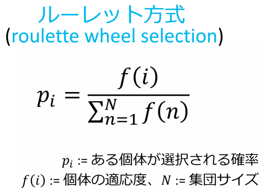
def select_roulette(generation):
'''選択の関数(ルーレット方式)'''
selected = []
weights = [ind.get_fitness() for ind in generation]
norm_weights = [ind.get_fitness() / sum(weights) for ind in generation]
selected = np.random.choice(generation, size=len(generation), p=norm_weights)
return selected
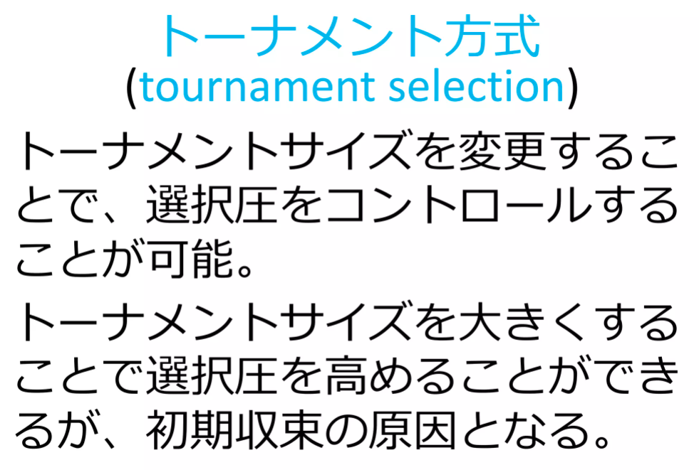
def select_tournament(generation):
'''選択の関数(トーナメント方式)'''
selected = []
for i in range(len(generation)):
tournament = np.random.choice(generation, 3, replace=False)
max_genom = max(tournament, key=Individual.get_fitness).genom.copy()
selected.append(Individual(max_genom))
return selected
def crossover(selected):
'''交叉の関数'''
children = []
if POPURATIONS % 2:
selected.append(selected[0])
for child1, child2 in zip(selected[::2], selected[1::2]):
if np.random.rand() < CROSSOVER_PB:
child1, child2 = cross_two_point_copy(child1, child2)
children.append(child1)
children.append(child2)
children = children[:POPURATIONS]
return children
def cross_two_point_copy(child1, child2):
'''二点交叉'''
size = len(child1.genom)
tmp1 = child1.genom.copy()
tmp2 = child2.genom.copy()
cxpoint1 = np.random.randint(1, size)
cxpoint2 = np.random.randint(1, size - 1)
if cxpoint2 >= cxpoint1:
cxpoint2 += 1
else:
cxpoint1, cxpoint2 = cxpoint2, cxpoint1
tmp1[cxpoint1:cxpoint2], tmp2[cxpoint1:cxpoint2] = tmp2[cxpoint1:cxpoint2].copy(), tmp1[cxpoint1:cxpoint2].copy()
new_child1 = Individual(tmp1)
new_child2 = Individual(tmp2)
return new_child1, new_child2
def mutate(children):
for child in children:
if np.random.rand() < MUTATION_PB:
child.mutate()
return children
def create_generation(POPURATIONS, GENOMS):
'''初期世代の作成
return: 個体クラスのリスト'''
generation = []
for i in range(POPURATIONS):
# individual = Individual(np.random.randint(0, 2, GENOMS))
individual = Individual(np.random.randint(0, 5, GENOMS))
generation.append(individual)
return generation
def ga_solve(generation):
'''遺伝的アルゴリズムのソルバー
return: 最終世代の最高適応値の個体、最低適応値の個体'''
best = []
worst = []
# --- Generation loop
print('Generation loop start.')
for i in range(GENERATIONS):
# --- Step1. Print fitness in the generation
best_ind = max(generation, key=Individual.get_fitness)
best.append(best_ind.fitness)
worst_ind = min(generation, key=Individual.get_fitness)
worst.append(worst_ind.fitness)
print("Generation: " + str(i) \
+ ": Best fitness: " + str(best_ind.fitness) \
+ ". Worst fitness: " + str(worst_ind.fitness))
# --- Step2. Selection (Roulette)
# selected = select_roulette(generation)
selected = select_tournament(generation)
# --- Step3. Crossover (two_point_copy)
children = crossover(selected)
# --- Step4. Mutation
generation = mutate(children)
print("Generation loop ended. The best individual: ")
print(best_ind.genom)
return best, worst
np.random.seed(seed=65)
# param
POPURATIONS = 100
# GENOMS = 50 # 江端修正
GENOMS = 160
GENERATIONS = 1000
CROSSOVER_PB = 0.8
MUTATION_PB = 0.1
# create first genetarion
generation = create_generation(POPURATIONS, GENOMS)
# solve
best, worst = ga_solve(generation)
# plot
fig, ax = plt.subplots()
ax.plot(best, label='max')
ax.plot(worst, label='min')
ax.axhline(y=GENOMS, color='black', linestyle=':', label='true')
ax.set_xlim([0, GENERATIONS - 1])
#ax.set_ylim([0, GENOMS * 1.1])
ax.set_ylim([0, GENOMS * 2.2])
ax.legend(loc='best')
ax.set_xlabel('Generations')
ax.set_ylabel('Fitness')
ax.set_title('Tournament Select')
plt.show()

明日は、この2つをマージして、目的のプログラムを完成させます。
以下のプログラムは、20個のデータを使って因子分析を行い、その分析因子分析を同じ結果を生み出す200個のダミーデータを作成します。
アルゴリズムの説明は省略します(が、私は分かっています)。
まず、データ(sample_factory.csv)
x1,x2,x3,x4,x5,x6,x7,x8
2,4,4,1,3,2,2,1
5,2,1,3,1,4,2,1
2,3,4,3,4,2,4,5
2,2,2,2,3,2,2,2
5,4,3,4,4,5,4,3
1,4,4,2,4,3,2,3
3,1,1,1,1,2,1,1
5,5,3,5,4,5,3,5
1,3,4,1,3,1,3,1
4,4,3,1,4,4,2,1
3,3,3,2,4,4,4,2
1,2,1,3,1,1,1,1
5,2,3,5,2,5,1,3
4,1,1,3,1,2,2,1
1,1,1,1,2,1,2,1
3,1,2,1,1,3,2,1
1,2,3,5,2,2,2,2
3,1,1,3,2,4,2,1
3,2,3,2,2,2,2,5
1,4,3,1,4,3,5,3
以下、GAのコード
# ebata@DESKTOP-P6KREM0:/mnt/c/Users/ebata/go-efa$ python3 ga-factory2.py

# ライブラリのインポート
import numpy as np
import pandas as pd
import matplotlib.pyplot as plt
# import japanize_matplotlibe
from factor_analyzer import FactorAnalyzer
import matplotlib.pyplot as plt

class Individual:
    '''各個体のクラス
        args: 個体の持つ遺伝子情報(np.array)'''
    def __init__(self, genom):
        self.genom = genom
        self.fitness = 0  # 個体の適応度(set_fitness関数で設定)
        self.set_fitness()

    def set_fitness(self):
        '''個体に対する目的関数(OneMax)の値をself.fitnessに代入'''
        # まずgenomを行列にデータに変換する
        # self.fitness = self.genom.sum()

        # 遺伝子列を行列に変換
        arr2d = self.genom.reshape((-1, 8)) # 列が分からない場合は、-1にするとよい

        # 各列の平均と標準偏差を計算
        mean = np.mean(arr2d, axis=0)
        std = np.std(arr2d, axis=0)

        # 標準偏差値に変換
        standardized_arr2d = (arr2d - mean) / std

        # 因子分析の実行
        fa_arr2d = FactorAnalyzer(n_factors=2, rotation="promax")
        fa_arr2d.fit(standardized_arr2d)

        # 因子分析行列の算出
        loadings_arr2d = fa_arr2d.loadings_

        # 因子分析行列の差分算出
        distance2 = euclidean_distance(fa.loadings_, loadings_arr2d)
        # print(distance2)

        # とりあえず評価関数をこの辺から始めてみる
        self.fitness = 1 / distance2

    def get_fitness(self):
        '''self.fitnessを出力'''
        return self.fitness

    def mutate(self):
        '''遺伝子の突然変異'''
        tmp = self.genom.copy()
        i = np.random.randint(0, len(self.genom) - 1)
        # tmp[i] = float(not self.genom[i])
        tmp[i] = np.random.randint(1, 6) #  江端修正
        self.genom = tmp
        self.set_fitness()


def euclidean_distance(matrix_a, matrix_b):
    # 行列Aと行列Bの要素ごとの差を計算します
    diff = matrix_a - matrix_b

    # 差の二乗を計算します
    squared_diff = np.square(diff)

    # 差の二乗の和を計算します
    sum_squared_diff = np.sum(squared_diff)

    # 和の平方根を計算します
    distance = np.sqrt(sum_squared_diff)

    return distance


def select_roulette(generation):
    '''選択の関数(ルーレット方式)'''
    selected = []
    weights = [ind.get_fitness() for ind in generation]
    norm_weights = [ind.get_fitness() / sum(weights) for ind in generation]
    selected = np.random.choice(generation, size=len(generation), p=norm_weights)
    return selected


def select_tournament(generation):
    '''選択の関数(トーナメント方式)'''
    selected = []
    for i in range(len(generation)):
        tournament = np.random.choice(generation, 3, replace=False)
        max_genom = max(tournament, key=Individual.get_fitness).genom.copy()
        selected.append(Individual(max_genom))
    return selected


def crossover(selected):
    '''交叉の関数'''
    children = []
    if POPURATIONS % 2:
        selected.append(selected[0])
    for child1, child2 in zip(selected[::2], selected[1::2]):
        if np.random.rand() < CROSSOVER_PB:
            child1, child2 = cross_two_point_copy(child1, child2)
        children.append(child1)
        children.append(child2)
    children = children[:POPURATIONS]
    return children


def cross_two_point_copy(child1, child2):
    '''二点交叉'''
    size = len(child1.genom)
    tmp1 = child1.genom.copy()
    tmp2 = child2.genom.copy()
    cxpoint1 = np.random.randint(1, size)
    cxpoint2 = np.random.randint(1, size - 1)
    if cxpoint2 >= cxpoint1:
        cxpoint2 += 1
    else:
        cxpoint1, cxpoint2 = cxpoint2, cxpoint1
    tmp1[cxpoint1:cxpoint2], tmp2[cxpoint1:cxpoint2] = tmp2[cxpoint1:cxpoint2].copy(), tmp1[cxpoint1:cxpoint2].copy()
    new_child1 = Individual(tmp1)
    new_child2 = Individual(tmp2)
    return new_child1, new_child2


def mutate(children):
    for child in children:
        if np.random.rand() < MUTATION_PB:
            child.mutate()
    return children


def create_generation(POPURATIONS, GENOMS):
    '''初期世代の作成
        return: 個体クラスのリスト'''
    generation = []
    for i in range(POPURATIONS):  # POPURATIONS = 100
        # individual = Individual(np.random.randint(0, 2, GENOMS))
        individual = Individual(np.random.randint(1, 6, GENOMS))
        generation.append(individual)
    return generation


def ga_solve(generation):
    '''遺伝的アルゴリズムのソルバー
        return: 最終世代の最高適応値の個体、最低適応値の個体'''
    best = []
    worst = []
    # --- Generation loop
    print('Generation loop start.')
    for i in range(GENERATIONS):
        # --- Step1. Print fitness in the generation
        best_ind = max(generation, key=Individual.get_fitness)
        best.append(best_ind.fitness)
        worst_ind = min(generation, key=Individual.get_fitness)
        worst.append(worst_ind.fitness)
        print("Generation: " + str(i) \
                + ": Best fitness: " + str(best_ind.fitness) \
                + ". Worst fitness: " + str(worst_ind.fitness))

        # --- Step2. Selection (Roulette)
        # selected = select_roulette(generation)
        selected = select_tournament(generation)

        # --- Step3. Crossover (two_point_copy)
        children = crossover(selected)

        # --- Step4. Mutation
        generation = mutate(children)

    print("Generation loop ended. The best individual: ")
    print(best_ind.genom)
    return best, worst


np.random.seed(seed=65)

# param
POPURATIONS = 100  # 個体数
# GENOMS = 50 # 江端修正

# GENOMS = 160 # GENの長さ
GENOMS = 1600 # GENの長さ 1つのデータが8個の整数からなるので、合計200個のデ0タとなる

GENERATIONS = 1000
CROSSOVER_PB = 0.8

# MUTATION_PB = 0.1
MUTATION_PB = 0.3 # ミューテーションは大きい方が良いように思える

# ファイルからデータの読み込み
df_workers = pd.read_csv("sample_factor.csv")
print(df_workers)

# 変数の標準化
df_workers_std = df_workers.apply(lambda x: (x-x.mean())/x.std(), axis=0)
print(df_workers_std)


# 固有値を求める(不要と思うけど、残しておく)
ei = np.linalg.eigvals(df_workers.corr())
print(ei)

print("因子分析の実行") # 絶対必要
fa = FactorAnalyzer(n_factors=2, rotation="promax")
fa.fit(df_workers_std)

# print(fa.loadings_) # これが因子分析の行列


# 因子負荷量,共通性(不要と思うけど、残しておく)
loadings_df = pd.DataFrame(fa.loadings_, columns=["第1因子", "第2因子"])
loadings_df.index = df_workers.columns
loadings_df["共通性"] = fa.get_communalities()

# 因子負荷量の二乗和,寄与率,累積寄与率(不要と思うけど、残しておく)
var = fa.get_factor_variance()
df_var = pd.DataFrame(list(zip(var[0], var[1], var[2])),
                      index=["第1因子", "第2因子"],
                      columns=["因子負荷量の二乗和", "寄与率", "累積寄与率"])
print(df_var.T)


# create first genetarion
generation = create_generation(POPURATIONS, GENOMS)

# solve
best, worst = ga_solve(generation)

# plot

#fig, ax = plt.subplots()
#ax.plot(best, label='max')
#ax.plot(worst, label='min')
#ax.axhline(y=GENOMS, color='black', linestyle=':', label='true')
#ax.set_xlim([0, GENERATIONS - 1])
#ax.set_ylim([0, GENOMS * 1.1])
#ax.legend(loc='best')
#ax.set_xlabel('Generations')
#ax.set_ylabel('Fitness')
#ax.set_title('Tournament Select')
#plt.show()
ga-factory2.py :200固体 主成分行列からの距離は、distance2(これが一致度) 評価関数は、この逆数を使っているだけ
ga-factory3.py :2000固体
以上